Calculation of Area

14. In ArcMap, view the kernels and isopleth files.

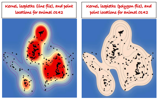
Determining AREA of home ranges

15. GME does not create a field in the attribute table of the polygon isopleth file indicating percent volume contours. The only field created in the polygon file is “ID”, but the records are all 0. To specify percent volume contour, select the first record, right-click on the ID field, and use the field calculator to input “95”. Repeat for the other contours.
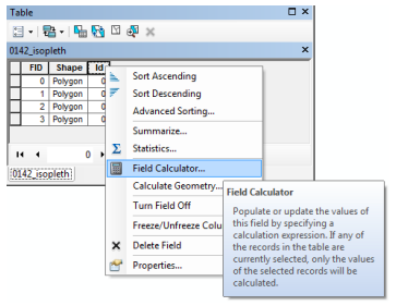
16. To determine area of each home range, add a new field in the attribute table by clicking the drop-down menu button in the upper left of the table and selecting “Add Field”. Name it “Area”. Specify the new field as a “FLOAT” with Precision of 10 and Scale of 2.
17. Once the new field is created, right-click on the field name in the attribute table, navigate to “Calculate Geometry”, and specify the appropriate units (e.g., hectares, square kilometers).
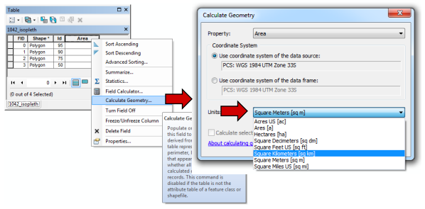
18. To determine the total area of the home range, right-click on the “Area” field and select “Statistics”. The sum of the area between each isopleth will be given.

Vegetation Analysis – Determining “Available” Habitat

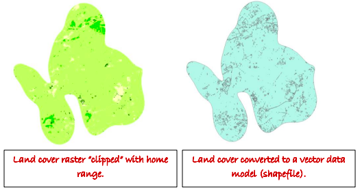
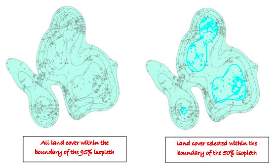
In ArcMap, at this point, you should have your isopleth shapefile of the home range for an individual animal, and a layer indicating vegetation type. In this example, we use a raster file depicting land cover and ultimately convert it to a vector shapefile for additional analyses. These spatial analyses may also be done using all rasters if you are familiar with raster analyses, but the methods will be different than those indicated below. For this analysis, we defined “available habitat” as the vegetation available within the boundaries of the home range. We analyzed available habitat for each percent volume contour (isopleth). For instance, the steps below describe how we determine available habitat in the area between the 90 and 95% isopleths.

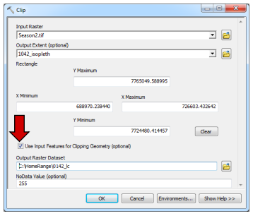
19. The land cover raster file obviously spans a larger spatial extent than an individual home range. To “Clip” the land cover raster with the extent of the home range, use the “Raster Clip” tool. Navigate to Data Management Tools → Raster → Raster Processing → Clip. Input is the land cover raster. The Output extent is the home range isopleth shapefile. BE SURE TO CHECK THE BOX SPECIFYING THAT YOU WANT TO “Use Input Features for Clipping Geometry”. Name the file something descriptive like 0142_lc.img (i.e., indicating animal ID 0142 and land cover).
20. Convert the clipped raster to vector by using a conversion tool. Navigate to Conversion Tools → From Raster → Raster to Polygon. Input is raster file from previous step (0142_lc.img). The “Field” input should be the “value” field or other field in the raster file indicating land cover types. Name the file something descriptive like 0142_lcov.shp (i.e., indicating animal ID 0142 and land cover).
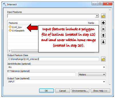
21. To create a shapefile indicating home range, isolines, and vegetation, you now must intersect the newly converted shapefile of vegetation (0142_lcov.shp) with the home range isopleth shapefile of the same individual (i.e., 0142isopleth.shp. See step 12). The “intersect” tool may be accessed by navigating to Analysis Tools → Overlay → Intersect. Input the 2 files. Name the output something descriptive such as 0142_intersect.shp.
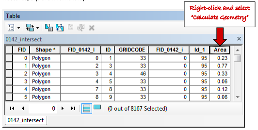
22. Now that you have a shapefile depicting percent volume contours (isopleths) and land cover within a home range, you are ready to determine the amount of area available between isopleths. Any time you perform a geoprocessing function such as an intersect, ArcMap does not automatically update area. To update area, open the attribute table for your shapefile of the land cover – isopleth intersection (i.e., 0142_intersect.shp). UPDATE the AREA FIELD by rightclicking the “Area” field and selecting “Calculate Geometry”. Choose appropriate units (e.g., hectares, square kilometers).
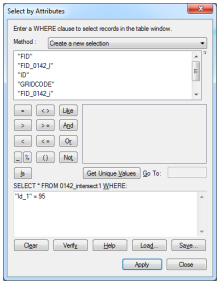
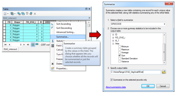
    NOTE: the sum of the AREA will exceed the total area of the home range because polygons are essentially duplicated if they occur within the smaller isopleths. For instance, polygons occurring in the area between the 50 and 75% isopleths ALSO occur within the area between 90-95% isopleths. DO NOT USE THE SUM OF THE AREA TO COMPUTE TOTAL HOME RANGE SIZE. Use steps 15-18 to determine home range area.
23. To effectively summarize the amount of area within each land cover category between isopleths, first conduct an attribute query to select the area you are interested in analyzing. For instance, conduct a query for all polygons in the 95% isopleth.
24. Next, Right-click the field indicating land cover type (in the example, land cover is indicated in the “GRIDCODE” field) and select “Summarize”. In the ”Summarize” dialog box, check the box next to “Sum” of “Area”. Save the output table as a *.txt file. Name it 0142_VegAvail95.txt. Saving the file with a *.txt extension will allow you to open the file in a spreadsheet such as Excel for further analysis. This table will indicate the total area available for each land cover type.

Vegetation Analysis – Determining “Used” Habitat

We assumed that “used” habitat was vegetation corresponding with the point locations of an animal.

25. To determine “used” habitat, you need the shapefile of point locations for an individual animal (i.e., ID_0142.shp; see step 4) and the shapefile of the intersection between land cover and home range (i.e., 0142_intersect.shp; see step 21.) Make sure both of those files are added to ArcMap.
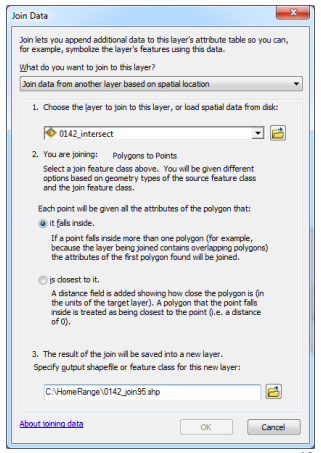
26. Determining “used” habitat requires conducting a spatial join between the point locations and the shapefile depicting land cover. To determine habitat used for locations occurring within the entire home range (i.e., between the 0 and 95% isopleths), right-click the point file in the Table of Contents, and select Joins and Relates  Join. Specify “Join attributes based on spatial location.” Join it to the intersected file. Name the output something like 0142_join95.shp to indicate a spatial join involving all points within the home range boundary. This step will create another shapefile indicating the vegetation type associated with each location.
27. In the resulting attribute table, conduct an attribute query to select all records in the 95% isopleth. Next, right-click on the field in the attribute table indicating land cover type (e.g., GRIDCODE) and select “Summarize”. None of the boxes need to be checked. This process will indicate the number of point locations occurring within each land cover class. Save the output table with a *.txt extension so you may open it in a spreadsheet. Name the output table something like 0142_VegUsed95.txt.
28. If you are analyzing habitat use within various isopleths, you must first isolate point locations occurring within isopleths. For instance, in this example, let’s determine land cover types used within the boundary of the 50% isopleth. Therefore, conduct an attribute query on the intersected shapefile (0142_intersect.shp) to select all records composing the area within the boundary of the 50% isopleth.
29. Next, in the Table of Contents, right-click the intersected shapefile and navigate to Selection → Create Layer From Selected Features. The new layer will be added to the top of the Table of Contents. If you would like to rename it, click the name of the layer, and then click once more. For instance, we can name the new layer something descriptive like “landcov50.” This process does NOT create a new shapefile, it simply isolates selected records from a shapefile.
30. Now, you can join the shapefile of point locations (ID_0142.shp) to the shapefile depicting vegetation within the boundary of the 50% isopleth by right-clicking the name of the point file in the Table of Contents and selecting Joins and Relates → Join. In the dialog box, specify “Join data from another layer based on spatial location”. Join it to the newly created layer, landcov50. Name the output 0142_join50.shp.
31. Summarize as in step 27. Continue obtaining “Used” data for each animal.